17 Real Interest Rates and the Taylor Rule
17.1 Real Interest Rates
We have described how central banks control short-term interest rates on interbank loans. We have also described how longer-term interest rates are affected by expectations about what will happen to short-term rates in the future. It is through this mechanism that central banks influence risk-free rates at all maturities.
Considerations about default risk and collateral then need to be factored in to understand movements in interest rates for risky private-sector lending. These private-sector interest rates have a significant effect on the economy: high interest rates negatively affect the economy by discouraging spending.
But what do we mean by a high interest rate? Is ten percent a high interest rate?
It depends on the level of inflation.
17.1.1 Real Interest Rates and Consumption
Real interest rates are calculated by subtracting the rate of inflation from the rate of interest, which is also known as the nominal interest rate. If the nominal interest rate is 10%, then if inflation is 10%, the real interest rate is zero. If inflation is 5%, the real interest rate is 5%.
Consider the decision to save for tomorrow or spend today. The argument for saving is that it can allow you to consume more tomorrow. If the real interest rate is negative, this means you will be able to purchase less tomorrow with the money that you set aside. For instance, if the interest rate is 5% but inflation is 10%, then you receive 5% in interest but your savings have eroded in value by more than that.
Thus, low real interest rates discourage saving and high real interest rates encourage it.
17.1.2 Real Interest Rates and Business Investment
Consider a firm that is thinking about buying capital equipment and suppose the interest rate is 10%.
- If the firm is borrowing the money, it needs to consider whether the investment will generate enough new profit income to justify paying back both the amount borrowed (the principal) and the interest.
- If the firm has spare money available, it needs to consider whether it would be better off putting the money in the bank at the prevailing interest rate rather than buying the machine.
Either way, the higher the interest rate, the less likely the firm is to buy the equipment. Again, inflation matters when thinking about whether an interest rate is considered high. If inflation is 10%, the firm can expect that its profits will be increasing by that much and a 10% interest rate will not seem so high. But if prices are falling, then a 10% interest rate on borrowings will seem very high.
Low real interest rates encourage business investment and high real interest rates discourage it.
17.2 The Taylor Rule
We have covered material that helps explain roughly how modern central banks should behave, including policies to influence interest rates and the implications of the expectations-augmented Phillips curve. But this does not address the basic operational question: How should a central bank decide what is the right interest rate to set at any point in time?
Here we discuss a famous monetary policy “rule,” first discussed in a 1993 paper by Stanford economist John Taylor. Much of the discussion of monetary policy today uses the so-called Taylor rule as a benchmark for how policy should be conducted. We will describe the rule and how it would be implemented, discuss how well it explains actual policy, and consider its relevance to current US monetary policy.
17.2.1 The Taylor Rule and Real Interest Rates
Taylor’s rule says that the Federal Reserve should set the federal funds rate according to the following formula:
\[ \begin{aligned} \text{Federal Funds Rate} = {}& \text{Inflation Rate} \\ & + 0.5(\text{Inflation Rate} - 2\%) \\ & + 0.5(\text{Gap Between Real GDP and Its Trend}) \\ & + 2\%. \end{aligned} \]
For example, if the inflation rate were 4% and the gap between real GDP and its trend level (known as the output gap) were minus 1%, the Taylor rule would recommend setting the federal funds rate equal to 6.5%, because
\[ 4 + 0.5(4-2) + 0.5(-1) + 2 = 6.5. \]
The “Inflation Rate minus 2%” term in the rule relies on the assumption that 2% is the Fed’s target rate of inflation. The idea of reacting to real GDP differing from its trend comes from the Phillips curve: above-trend values of GDP may signal an increase in inflation, while below-trend values may signal a fall in inflation.
Note that when inflation goes up, the rule says that the federal funds rate should go up by more. Specifically, a one-percentage-point increase in inflation should be matched by a 1.5-percentage-point increase in the federal funds rate.
This means there is an increase in the real interest rate when inflation rises. The real interest rate is the actual, or nominal, interest rate set by the Fed minus inflation.
Taylor had a very specific recommendation for how the Fed should respond to inflation: raise the federal funds rate by 1.5 percentage points for every one-percentage-point increase in inflation. But the general idea that policy rates should change by more than the change in inflation is now known as the Taylor principle.
Let’s See If You Understand the Taylor Principle
A central bank responds to inflation rising from 2 percent to 3 percent by increasing the policy interest rate from 1 percent to 2.5 percent. Does this action conform to the Taylor principle?
Inflation rose from 2% to 3%, so it increased by one percentage point. The policy interest rate rose from 1% to 2.5%, so it increased by 1.5 percentage points. The policy interest rate rose by more than the inflation rate, so yes, this action satisfies the Taylor principle.
17.2.2 The Fed and the Taylor Principle
Many studies of the so-called Great Inflation of the 1970s argue that the Fed did not obey the Taylor principle during that decade. They allowed real interest rates to fall when inflation rose, which further fueled inflation. This lack of responsiveness of policy to inflation helps explain why inflation became so high during the 1970s.
Historical evidence, such as Allan Meltzer’s History of the Federal Reserve, points out that there was little discussion at the Fed of the concept of real interest rates during the 1970s until Paul Volcker became chair. Estimates of the responsiveness of the federal funds rate to inflation since 1979 are significantly higher than in the prior period.
Other researchers have pointed to the uncertainty in estimates of the output gap at the time as a complicating factor. The Fed continually mistook what was a permanent slowdown in average growth rates for a transitory one.
This shows one drawback of the Taylor rule: it requires an estimate of the gap between output and its “non-inflationary” potential level. In practice, obtaining estimates of this gap is fraught with difficulties.
17.2.3 The Long-Run Real Interest Rate
Recall the original Taylor rule:
\[ \begin{aligned} \text{Federal Funds Rate} = {}& \text{Inflation Rate} \\ & + 0.5(\text{Inflation Rate} - 2\%) \\ & + 0.5(\text{Output Gap}) + 2\%. \end{aligned} \]
The number 2% features twice in Taylor’s rule, representing two different concepts. As well as the “Inflation Rate minus 2%” term, the rule contains the “+2%” element at the end.
How should this second term be interpreted? Suppose the gap between GDP and its trend were zero and inflation equaled the Fed’s target of 2%. Then the federal funds rate would equal 4% and the real interest rate would be 2%.
Since the rule was designed to deliver average inflation of zero and since GDP should on average equal its trend, this meant Taylor was recommending an average long-run real interest rate of 2%.
17.3 An Updated Implementation of the Taylor Rule
Since Taylor’s paper, there has been a great deal of additional research on monetary policy rules. In May 2009, Glenn Rudebusch of the Federal Reserve Bank of San Francisco published a paper with a “Taylor rule” constructed to match the average behavior of the Fed over the period 1988 to 2008.
Rudebusch used core consumer prices to measure inflation and an unemployment gap instead of an output gap. This unemployment gap was constructed as the difference between the unemployment rate and the Congressional Budget Office’s (CBO) estimate of the so-called natural rate of unemployment.
Estimating the relationship with data from 1988 to 2008 gives the following rule:
\[ \begin{aligned} \text{Federal Funds Rate} = {}& 0.75 + 1.75(\text{Core Inflation}) \\ & - 1.71(\text{Unemployment Gap}). \end{aligned} \]
This rule implied that there should have been highly negative federal funds rates during the global financial crisis and again during the COVID pandemic. The lecturer updated this rule using monthly data through October 2023.
Figure 1. Glenn Rudebusch’s Taylor Rule
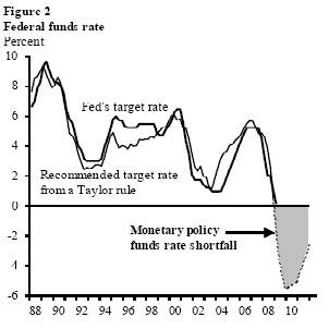
Source: Rudebusch (2009).
Figure 2. Unemployment Gap and Core Inflation: Inputs into the Rudebusch Taylor Rule
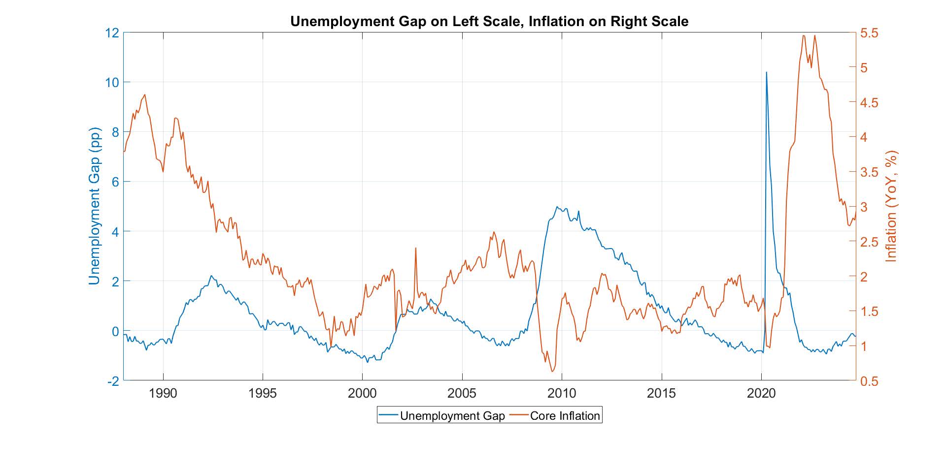
Source: Author’s calculations based on data from the St. Louis Fed.
Figure 3. Updated Rudebusch Taylor Rule: Actual Federal Funds Rate and Predicted Rate
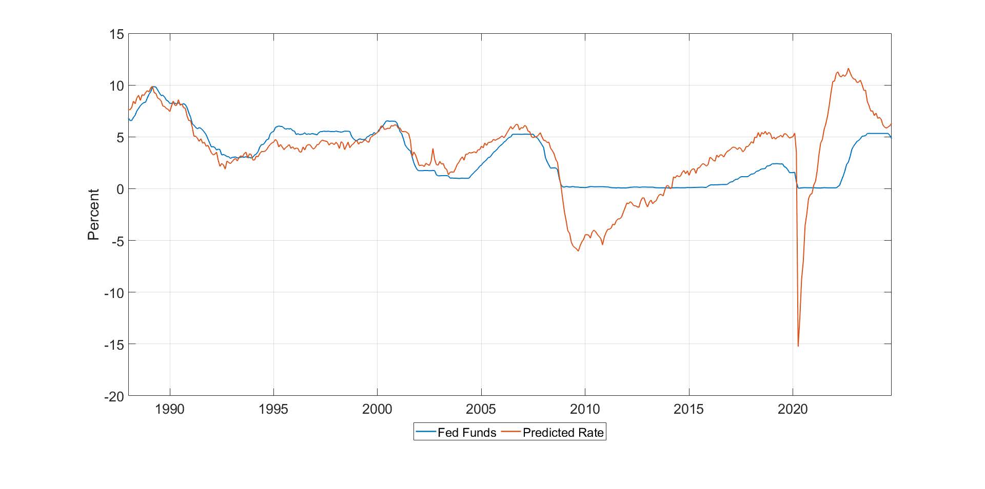
Source: Author’s calculations based on data from the St. Louis Fed.
17.3.1 How Constraining Was the Zero Bound?
The Fed has never cut the federal funds rate below zero. Our update of Rudebusch’s graph suggests that this stopped the Fed from implementing rates consistent with the Taylor rule during and after the global financial crisis, and also during the pandemic. After the financial crisis, the federal funds rate suggested by the rule remained negative until early 2014. During the global pandemic, the rule again suggested that the funds rate should have been slashed to minus 12%.
This makes it look as though the zero bound seriously constrained the Fed. But looks can be deceiving. A 2018 paper by Eric Swanson pointed out that even when the Fed kept its policy rate at zero, it was able to move long-term rates—which matter more for the economy—through quantitative easing and forward guidance. Swanson suggested that the responsiveness of long-term interest rates to economic news did not change much during the period when the federal funds rate was zero. This suggests that the Fed was still able to convince markets it had the tools to influence the economy.
17.4 The Fed and the Taylor Rule Prior to 2020
In the years prior to the pandemic, the Fed had clearly departed from following the Taylor rule. The Taylor rule’s recommended policy rate turned positive in late 2013, but the Fed did not raise rates above zero until 2016. It then started cutting rates in 2019, when the rule suggested keeping them stable at a higher level.
We will focus on two reasons why the Fed departed from the Taylor rule: lower long-run real interest rates and less concern about inflation.
17.4.1 Lower Long-Term Average Real Rates
Recall Rudebusch’s rule:
\[ \begin{aligned} \text{Federal Funds Rate} = {}& 0.75 + 1.75(\text{Core Inflation}) \\ & - 1.71(\text{Unemployment Gap}). \end{aligned} \]
From this, we can calculate that the long-run average real interest rate consistent with 2% inflation is 2.25%, because
\[ 2.25 = 0.75 + 1.75\times 2 - 2. \]
However, Fed officials do not believe the average real interest rate in the future will be this high. FOMC members provide forecasts for macroeconomic variables such as inflation and for the federal funds rate, including a “longer-run” forecast.
In January 2012, the FOMC’s median estimate of the long-run real federal funds rate was 2.25%. In recent years, this estimate has been 0.5%. This implies that they think interest rates should be 1.75 percentage points lower on average now than in the past.
Why? Macroeconomists now largely agree that equilibrium real interest rates are lower than they used to be, with various explanations offered, including demographics and weak productivity growth.
17.4.2 Less Concern About Inflation
The idea of raising interest rates when unemployment is low, or the output gap is positive, rests on the Phillips curve: the idea that low unemployment signals higher future inflation.
However, in the years prior to the pandemic, inflation was consistently low in advanced economies despite many of them experiencing low unemployment for extended periods of time.
Many speculated that “the Phillips curve is dead,” so central banks no longer needed to worry about economies overheating and generating higher inflation. By 2020, the Fed had made clear that it had decided to keep interest rates low as long as inflation remained contained and to stop worrying about the potential inflationary implications of low unemployment.
In a reformulation of its monetary policy, the Fed said that it would worry less about strong labor market conditions than it had previously. In August 2020, Fed Chair Powell said that under the new approach to monetary policy,
“employment can run at or above real-time estimates of its maximum level without causing concern, unless accompanied by signs of unwanted increases in inflation.”
17.5 High Inflation and Monetary Tightening
After many years of low inflation, the world suddenly had plenty of “unwanted inflation” in 2021. Inflation in all advanced economies increased in 2021 and exceeded 10% in some countries in 2022. Inflation was driven both by strong aggregate demand, partly due to expansionary policies during the pandemic, and by large increases in food and energy prices due to the war in Ukraine.
Central banks responded by raising policy interest rates, but by much less than the Taylor rule would recommend. Why did they not increase rates by more?
- First, central banks anticipated that the effect of war-related supply shocks on inflation would quickly ease.
- Second, they were concerned that a global recession might be approaching, implying falling inflation.
- Third, the real interest rate that matters for the economy is probably not the short-term policy rate minus the current backward-looking measure of inflation. Longer-term real rates—defined as long-term rates minus expected inflation—did increase.
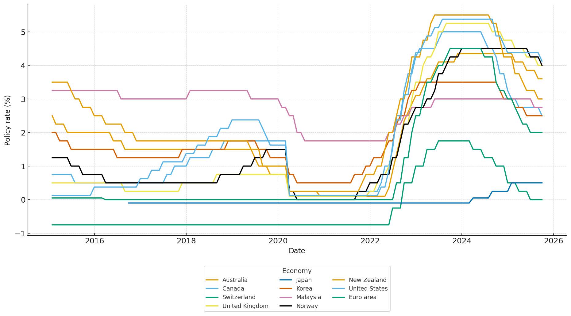
Figure 4. Monetary Policy Rates Around the World