15 Quantitative Easing

15.1 What is QE and How Is It Implemented?

We have already made references to Quantitative Easing (QE):

We stated that QE had produced a huge increase in the supply of reserve balances that banks hold with central banks.
We also noted that this big increase in reserves required central banks to adopt new approaches to implementing monetary policy, making the interest rate paid on reserves the new effective policy rate.

But we did not say what QE was. While the term “QE” is widely used in popular discussion, it is actually a pretty poor name for this and most central banks don’t use it.

QE is simply large scale open market operations involving asset purchases by central banks. The purchases are paid for via credits to reserve accounts of commercial banks.

Typically, central banks announce a set schedule of asset purchases that they are going to undertake. For example, the Fed may say they are going to purchase $50 billion of Treasury securities each month for a period. Let’s take a look at how QE programmes have affected the balance sheets of the Fed and Euro-system.

15.1.1 The Fed’s QE

The Federal Reserve first implemented a QE programme in late 2008 during the global financial crisis. From then until June 2010, they purchased $2.1 trillion dollars in mortgage-backed securities and US Treasury bonds. Further rounds of QE occurred November 2010 and June 2011, between September 2012 and October 2014 and during the global pandemic period.

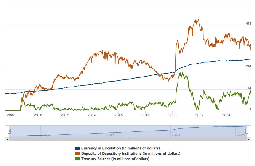
These asset purchases led to a huge increase in the Fed’s balance sheet relative to prior to 2008. The chart below illustrates how the Fed paid for these asset purchases. With each round of QE, there was a huge increase in the amounts that commercial banks held in reserve accounts with the Fed (denoted as “deposits of depository institutions” by the Fed).

The Fed is now very gradually reducing its asset holdings, taking payment on maturing assets. It is not actively selling securities.

Figure 1. The Fed’s Assets

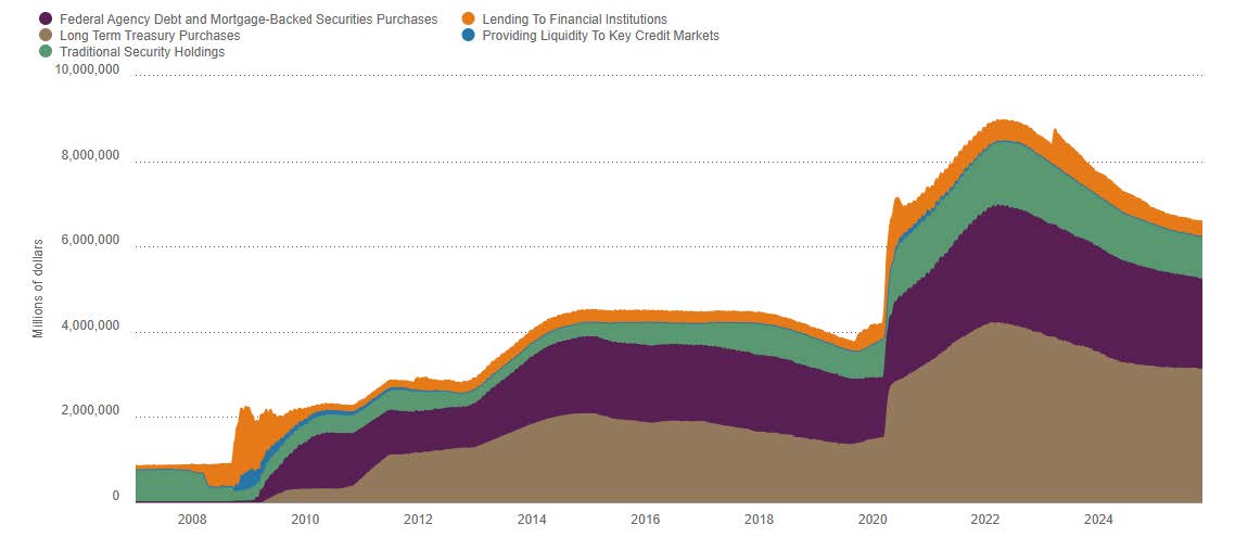
Figure 2. How the Fed Created Money via QE: currency in circulation, deposits of depository institutions, and Treasury balances .

Figure 15.2: How the Fed Created Money via QE

15.1.2 The Eurosystems’s QE

The ECB did not implement QE during either the global financial crisis of 2008/09 or the Euro crisis period of 2010 to 2012. Only in 2015 did the ECB implement an “Asset Purchase Programme” (APP) in response to inflation being persistently below its 2 percent target.

The APP saw each of the central banks and the ECB buying assets. The ECB bought 8 percent of the assets and the other 92 percent were bought by national central banks in proportion to their “capital key” (an average of their share in the euro area’s population and their share in GDP).

The APP bought some privately-issued bonds but mainly bought government securities, with each national central bank only buying securities issued by their own national government.

From March 2020 to March 2022, there was a “Pandemic Emergency Purchase Programme” (PEPP) with purchases of € 1.8 trillion in assets.

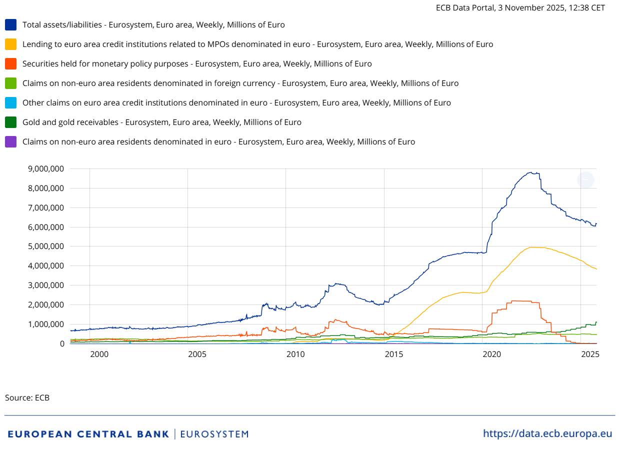
Like the Fed, the Eurosystem is now very gradually reducing its asset holdings, taking payment on maturing assets and not actively selling securities.

Figure 3. The Eurosystem’s Assets, in millions of euros

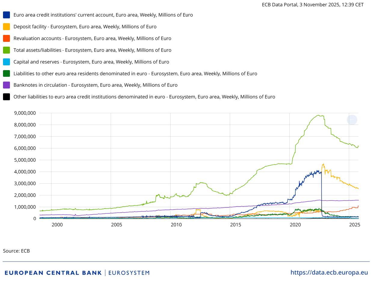
Figure 4. The Eurosystem’s Liabilities, in millions of euros

Figure 15.4: The Eurosystem’s Liabilities

15.2 Why Do Central Banks Implement QE?

Central banks implement QE to reduce long-term yields in important financial markets such as the markets for government bonds and mortgage-backed securities. They hope that by lowering these key benchmark rates, interest rates on other types of borrowing will also fall.

They also hope these interventions, by lowering bond yields, will increase asset prices and this will boost spending in the economy.

Let’s discuss how central banks think QE can influence bond yields.

15.2.1 Can Central Banks Influence Other Interest Rates?

Even when short-term money-market interest rates are zero or negative, important borrowing rates, such as mortgage rates, may still be positive. What can central banks do to reduce these rates?

As discussed previously, central banks can seek to lower long-term risk-free interest rates by signalling to financial markets that they intend to keep short-term interest rates low for a long time. Most major central banks have used this approach at some point over the past decade. This is the mechanism of forward guidance.

According to the models developed earlier in the course, however, there would seem to be no other mechanism. Our framework so far has been:

\[ \begin{aligned} \text{N-Year Risky Lending Rate} &= \text{N-Year Risk-Free Rate} \\ &\quad + \text{Risk Premium}. \end{aligned} \]

The N-year risk-free rate is determined by expected future short-term interest rates, while the risk premium depends on default risk and the quality of collateral. In that framework, these components determine the bond yield completely. In practice, however, interest rates can also be affected through mechanisms that this formula does not capture.

15.2.2 Why There Is a Demand Curve for Bonds

The “Risk Free Rate Plus Default Risk” formula effectively assumes that all investors are the same and would only hold a bond if it delivers the interest rate set by this formula.

In practice, things are a little different. Consider, the case of a bond that was yielding 3% and then, ceteris paribus, it started to yield 2% (The bond price goes up).

Demand for this bond would fall:

All investors have to make a trade-off between risk and return but investors differ in their willingness to take risks. Some investors that may have been comfortable with the risk-return tradeoff when the bond yielded 3% but now view it as too risky at 2%.
Investors may differ in their assessment of default risk. At 3% some may have viewed the bond as better value than a risk-free bond. At 2% some of these people may change their mind and view it as worse value.

What we are describing here is a demand curve. As the price of the bond goes up (yield goes down) there is less demand for it.

15.2.3 How QE Might Work: Supply and Demand for Bonds

How are bond prices determined? If the supply of a particular bond is fixed, and demand is greater at lower prices (higher yields), its equilibrium price equates the quantity supplied and the quantity demanded.

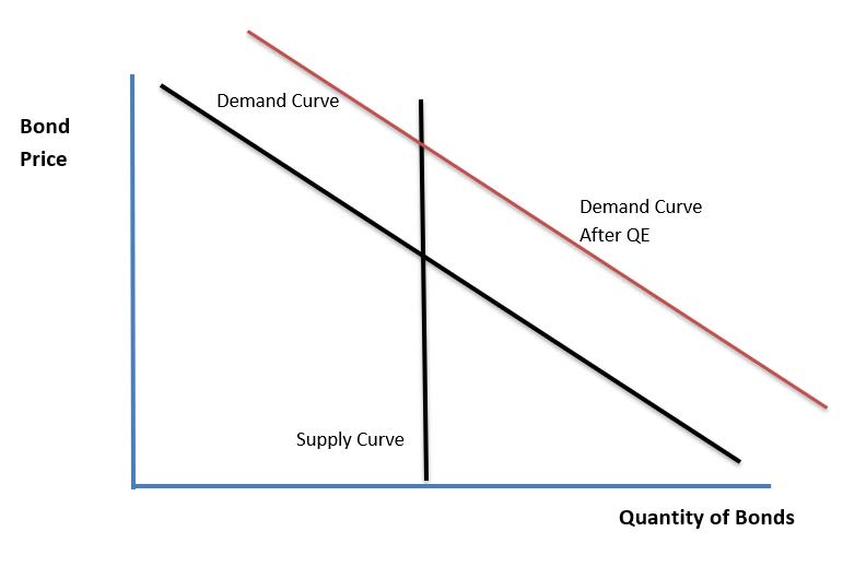
This provides another channel through which central banks can influence yields on a particular class of bonds. When a central bank purchases a specified quantity of a specified type of bond, its purchases shift the demand curve for that bond outward. The higher demand raises the bond’s price and lowers its yield. Equivalently, one can say that the private-sector demand curve remains unchanged, but the supply of bonds available to the private sector shifts inward, raising the price.

In actual markets, bond prices are not literally set by two curves crossing. Brokers continuously match buyers and sellers, and prices change from second to second. Nevertheless, the underlying principle remains: when demand to buy bonds is strong, brokers raise prices to induce investors to sell, and the resulting increase in bond prices reduces yields.

Figure 5. A Demand Curve for Bonds.

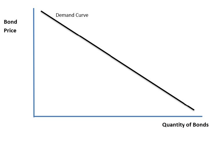
Figure 6. Bond Prices Set by Supply and Demand .

Figure 15.6: Bond Prices Set by Supply and Demand

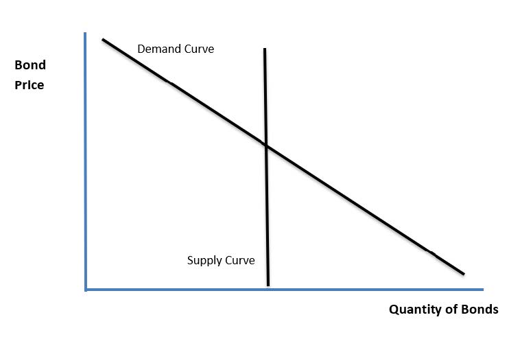
Figure 7. QE Increasing Bond Prices and Reducing Yields: an outward shift in demand

Figure 15.7: QE Increasing Bond Prices and Reducing Yields

15.2.4 An Example of How Bond Buying Works

It can be hard to find “clean” examples of how QE bond buying works.

Interest rates tend to move lower after QE but this could be because QE purchases send a signal that policy rates are going to be lower, i.e. it acts as a kind of forward guidance.

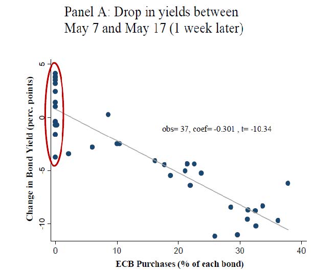
Below shows a picture from a great research paper by Christoph Trebesch and Jeromin Zettelmeyer that helps to answer this question. It shows the change in yields for a set of Greek government bonds between May 7, 2010 and May 17, 2010. This is when the ECB began purchasing Greek bonds with its Securities Market Program.

The data points circled by the red line correspond to bond issues that were not purchased by the ECB, while the rest of the data points correspond to bonds that had some ECB purchases.

The striking result is that only bonds that were purchased by the ECB saw falling average yields. And the more the ECB bought, the more the yields fell.

Figure 8. How ECB Bond Purchases Affected Greek Bond Yields: changes in yields against ECB purchases as a percentage of each bond

Figure 15.8: How ECB Bond Purchases Affected Greek Bond Yields

15.2.5 Evidence on the Effects of the Fed’s QE

Given uncertainty about how it works (Ben Bernanke joked “The problem with QE is it works in practice, but it doesn’t work in theory”) were Fed officials right to believe the QE programmes have an effect?

Bernanke summarises the evidence on the impact of QE from Ihrig et al (2018) as follows:

“QE1 reduced the 10-year term premium by 34 basis points, the Maturity Extension Program reduced term premiums by an additional 28 basis points, and QE3 reduced term premiums yet more, by 31 basis points on announcement and more over time.”

In other words, about $3.5 trillion dollars worth of money created to buy long-term bonds managed to reduce long-term yields by less than one percentage point. So while QE programmes can have an impact on interest rates, it is clear that it takes very large amounts of “money printing” in the form of QE to obtain a relatively small impact on long-term rates.

15.3 QE-Related Myths and Controversies

There are a lot of misunderstandings and myths around QE. Here, We will discuss:

QE as “Pumping money into banks to increase lending.”
QE boosting bank profits.
QE as a form of debt monetisation.
How QE has influenced recent developments for central bank profits.

15.3.1 QE and Bank Lending

Historical documents show that Ben Bernanke, the Fed chair who introduced QE, did not believe that QE would boost bank lending. The following statements from Federal Open Market Committee (FOMC) meetings illustrate these views.

“The Japanese approach, the quantitative easing approach, was focused on the liability side of the balance sheet—specifically the quantity of bank reserves, the monetary base, or however you want to put it, in the system.

The theory behind quantitative easing was that providing enormous amounts of very cheap liquidity to banks would encourage them to lend and that lending, in turn, would increase the broader measures of the money supply, which in turn would raise prices and stimulate asset prices, and so on, and that would suffice to stimulate the economy.

… I think that the verdict on quantitative easing is fairly negative. It didn’t seem to have a great deal of effect, mostly because banks would not lend out the reserves that they were holding. The one thing that it did seem to do was affect expectations of policy rates because everyone understood it would take some time to unwind the quantitative easing. Therefore, that pushed out into the future the increase in the policy rate.”

Fed Economists Joe Gagnon stated on QE at the March 2009 FOMC Meeting:

“A memo circulated to the FOMC last December reviewed the economic literature on this question and reported that a Federal Reserve purchase of $500 billion of long-term Treasury securities could plausibly reduce the 10-year Treasury yield by 20 to 100 basis points. Such a purchase would also be expected to lower long-term private yields. Generally speaking, public and private long-term debt markets are closely linked, and correlations of changes in yields across these markets have historically been very high.”

Dave Reifschneider stated:

“The top panel of your next exhibit reviews the basic channels through which buying agency MBS or long-term Treasury securities potentially influences the real economy. The primary mechanism is through a broad improvement in financial conditions. As Joe discussed, such purchases reduce yields on the targeted securities. In addition, the evidence suggests that these reductions spill over to yields on corporate bonds and other long-term instruments; if so, these interest rate movements should spark higher equity prices and a lower real exchange rate. In turn, household spending, business investment, and net exports should strengthen in response to lower borrowing costs, higher wealth, and greater international price competitiveness.”

Actually, the money multiplier slumped when the Fed introduced QE because banks did not increase their lending by much at the time. And staff briefings about QE at the time indicated the point of the policy was that it would lower long-term Treasury and mortgage rates.

15.3.2 QE and Bank Profits

Some commentators claim that QE is a programme intended to benefit banks. They may know that QE involves the Fed crediting the accounts commercial banks hold with it, but overlook the rest of the transaction.

As discussed earlier in the course when examining open market operations, banks are neither better nor worse off simply because of these operations. They acquire an additional asset in the form of reserves held at the central bank, but also acquire an additional liability in the form of a deposit owed to the person who sold the security to the central bank (as in the earlier example involving Janet).

Furthermore, for much of the period discussed in the lecture during which QE programmes operated, banks earned zero interest on their reserves. The lecturer’s conclusion is that QE was not a “secret bailout” for banks.

15.3.3 QE as Stealth Fiscal Policy

Others argue that QE is a form of debt monetisation—a hidden fiscal policy under which the government is financed by money created by the central bank. Such a description could apply if central banks directly purchased newly issued government bonds from the government.

However, the major central bank QE programmes discussed here involved purchases of securities in secondary markets. Central banks bought government-issued bonds from private-sector holders. Thus the private sector initially financed government borrowing, even though the central bank subsequently became the holder of the bonds.

QE clearly has some fiscal effects:

It lowers the interest rate on government debt, making it easier to spend more or tax less.
The interest payments on bonds owned by the central bank boost its profits and get returned to central government, lowering the net interest cost of the debt.

But conventional monetary policies also have fiscal consequences so this isn’t a new thing.

15.3.4 QE and Central Bank Profits Today

QE was introduced at a time when policy rates were zero around the world. Today, when policy rates are much higher, the combination of higher policy rates, large bond holdings by central banks and a large supply of commercial bank reserves is having negative fiscal consequences.

The bonds acquired during the QE programmes typically had low yields.
Because QE has only been very partially unwinded, there is still a very large supply of reserves.
And central banks are paying interest on reserves at their policy rate.

This means the cost of paying interest on reserves is exceeding the interest earned on the bonds acquired during QE. Central banks, which had made large profits over the previous decade, are now losing money which means they are not passing profits back to central governments anymore. In some cases, the magnitudes of this effect is large. One option to reduce this cost would be to use tiering when paying interest on reserves: Pay interest on the marginal reserves but not on all reserves. We know from the negative rate era that this works to set market rates, so why implement monetary policy in a way that has higher fiscal costs?