16 The Phillips Curve: Evidence and Implications
16.1 Central Banks and Economic Conditions
Modern economists tend to see inflation as being determined not by the money supply but by the overall demand for goods and services being strong relative to the economy’s capacity to supply them.
Central banks play an important role in influencing the demand for goods and services by controlling interest rates and credit conditions.
Lower interest rates can:
- Give more disposable income to those who have borrowed money, allowing them to spend more on goods and services.
- Make households, businesses, and governments more likely to borrow money for consumption or investment purchases.
- Increase the value of assets such as shares and houses,
- Increase lending from banks because credit risk for borrowers is lower when interest rates are low.
Central banks can also directly affect the supply of credit through macro-prudential policies. Through all of these channels, central banks can influence inflation.
16.2 Phillips curve
How does economic strength translate into inflation?
An early version of this idea was the so-called Phillips curve, named after LSE economist A. W. Phillips, who published a paper on the subject in 1958. The idea behind the Phillips curve was that inflation would be high when the unemployment rate was low, and inflation would be low when unemployment was high.
- The proposed mechanism starts when the economy is doing well and there is substantial demand for goods and services. Employers hire more workers, and the unemployment rate becomes low.
- Workers are then in high demand and can obtain higher wage increases.
- These increases in wage costs raise costs for firms, resulting in higher price inflation.
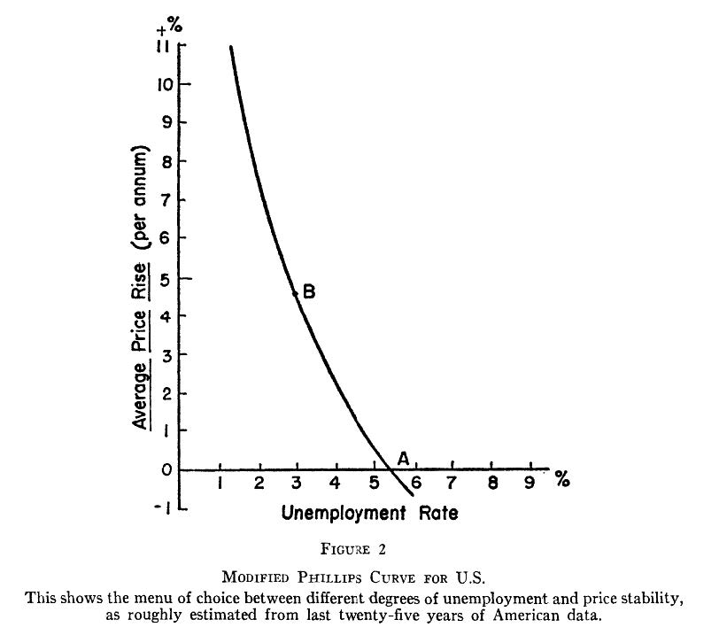
A 1960 study by MIT economists Solow and Samuelson replicated these findings for the United States and emphasised that the relationship also worked for price inflation. The Phillips curve tradeoff quickly became the basis for discussions of macroeconomic policy.
Figure 1. A. W. Phillips’s original relationship between money-wage inflation and unemployment, 1861–1913
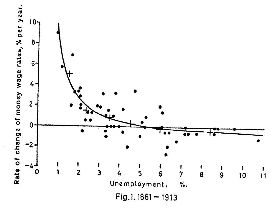
Figure 2. Phillips’s curve fitted to data for 1948–1957, with unemployment lagged seven months
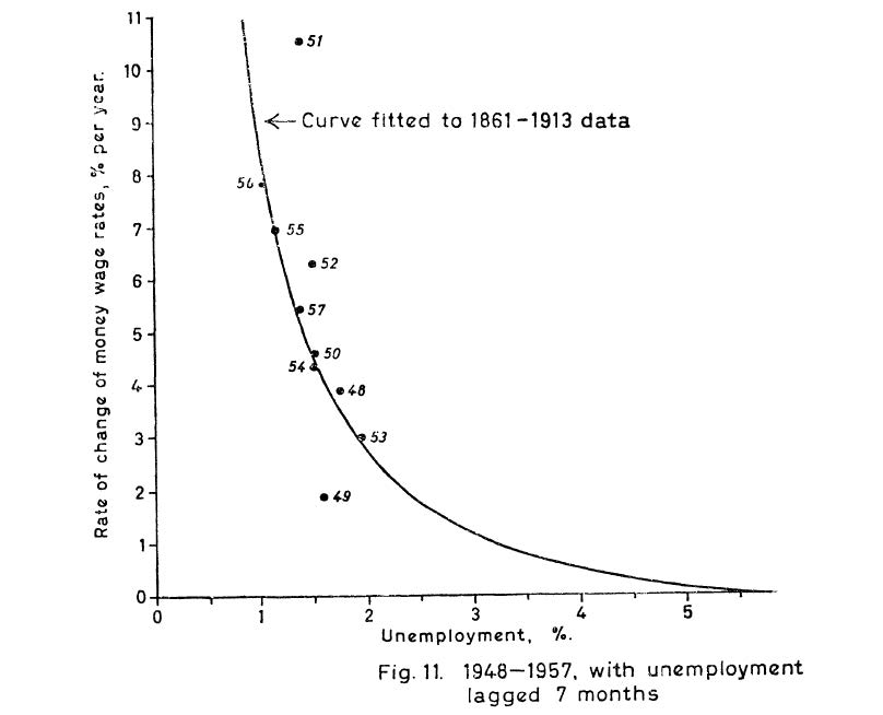
Figure 3. Solow and Samuelson’s modified Phillips curve for the United States, illustrating the proposed choice between unemployment and price stability
16.3 The Expectations-Augmented Phillips Curve
In a famous presidential address to the American Economics Association, Milton Friedman (1968) pointed out that it was expected real wages that affected wage bargaining.
If low unemployment gives workers a strong bargaining position, then high nominal wage inflation alone is not enough. Workers want nominal wage inflation to exceed price inflation.
Assuming that wage inflation is passed through to price inflation, this gives the expectations-augmented Phillips curve:
\[ \pi_t = \pi_t^e - \gamma(U_t-U^*) \]
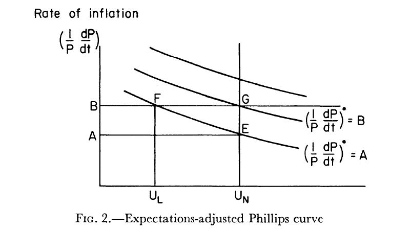
Friedman argued that if policy-makers tried to exploit an apparent Phillips curve tradeoff, the public would become accustomed to high inflation and come to expect it. Expected inflation, \(\pi_t^e\), would drift upwards, worsening the tradeoff between inflation and output.
In the long run, policy-makers cannot fool the public: \(\pi_t^e \approx \pi_t\). As a result, unemployment cannot be kept away from its natural rate, so \(U_t\approx U^*\).
Figure 4. Friedman’s expectations-adjusted Phillips curve, showing how higher inflation expectations shift the curve
16.4 The Demise of the Basic Phillips Curve
US monetary and fiscal policies in the 1960s were very expansionary. At first, the Phillips curve seemed to work: inflation rose, and unemployment fell. However, as the public became accustomed to high inflation, the Phillips curve tradeoff worsened. By the late 1960s, inflation was still rising even though unemployment had also increased.
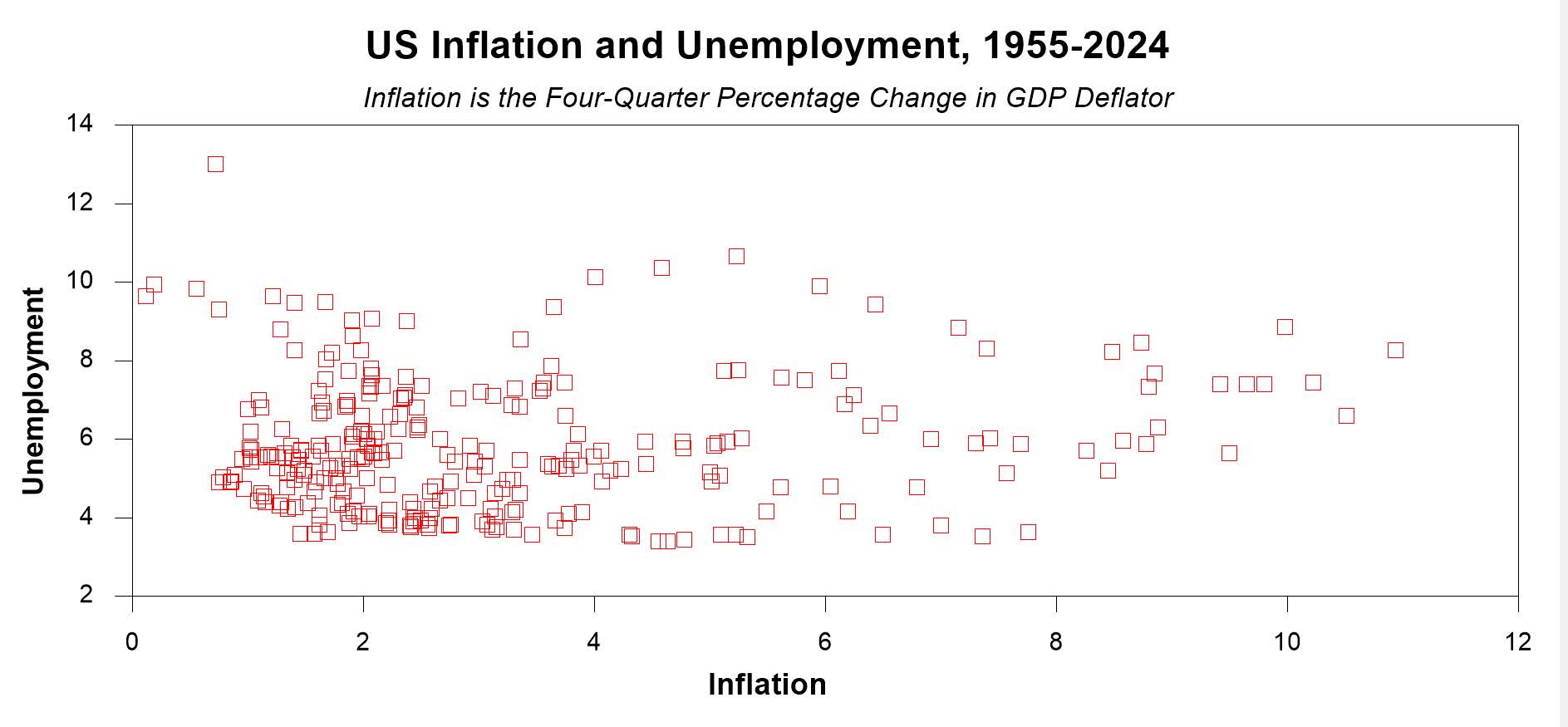
This combination of high inflation and high unemployment, known as stagflation, became even worse in the 1970s. This was exactly what Friedman had predicted. The data no longer show any clear negative relationship between inflation and unemployment, and the original formulation of the Phillips curve is widely regarded as wrong. The 1960s are now seen as an example of what can go wrong when monetary policy pursues the wrong goals.
Figure 5. US inflation and unemployment, 1955–2024
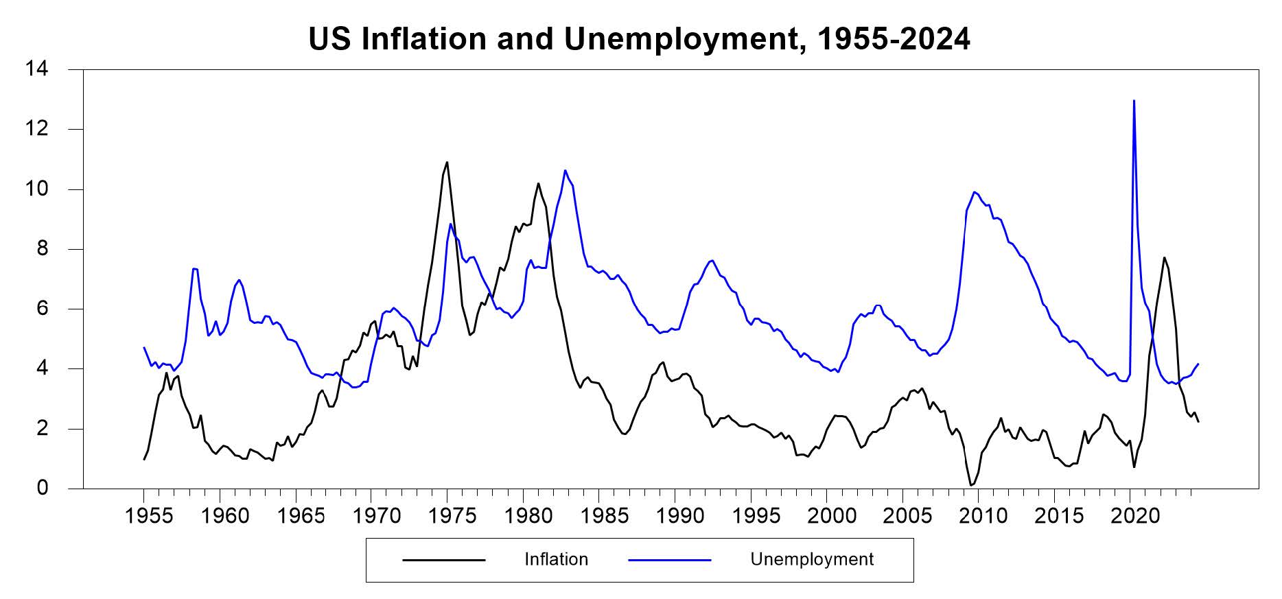
Figure 6. US inflation and unemployment, 1955–2024: the scatterplot does not show the stable negative relationship implied by the basic Phillips curve. Inflation is measured by the four-quarter percentage change in the GDP deflator
16.5 The Accelerationist Phillips Curve
What determines inflation expectations? Friedman argued that they are determined adaptively. For example, people might use last year’s inflation rate as a guide to what to expect this year. In that case, \(\pi_t^e = \pi_{t-1}\), and the expectations-augmented Phillips curve becomes
\[ \pi_t = \pi_{t-1} - \gamma(U_t-U^*) \]
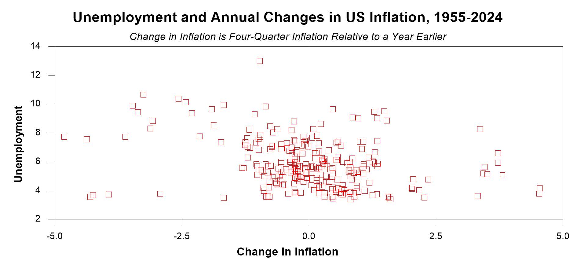
This equation relates the change in inflation to the gap between unemployment and its natural rate. When unemployment is below its natural rate, inflation will be increasing; when unemployment is above its natural rate, inflation will be decreasing. Because the model relates the rate of acceleration of the price level to unemployment, it is known as the accelerationist Phillips curve. This model fitted the data quite well for a long time.
Figure 7. Unemployment and annual changes in US inflation, 1955–2024. Inflation changes are measured as the change in four-quarter inflation relative to a year earlier
The accelerationist Phillips curve, relating changes in inflation to the unemployment rate, appears to offer a key tool to central bankers, and it is indeed useful. However, the real world is more complicated than this simple model. Two complications are particularly important:
16.5.1 Supply Shocks
Supply shocks, such as large increases or decreases in food or energy prices, can temporarily shift the inflation–unemployment tradeoff. In this case, the equation becomes
\[ \Delta\pi_t=-\gamma(U_t-U^*)+s_t \]
Bad supply shocks are those that raise inflation even though the unemployment rate has not changed. Oil-price shocks are a good example.
16.5.2 The natural rate of unemployment
The natural rate of unemployment, \(U^*\), is not a universal constant. It probably changes over time, and central bankers must estimate it at any particular moment. For example, the natural rate in Europe rose substantially in the 1980s and 1990s. More generally, central bankers are usually uncertain about how fast the economy can grow without triggering inflationary pressures.
16.5.3 Tradeoffs Offered by the Accelerationist Phillips Curve
Over the short term, the accelerationist model describes a new tradeoff for central bankers. For example, they can choose to keep unemployment below the natural rate temporarily at the expense of increasing inflation. However, the model does not really offer an exploitable long-run tradeoff.
Even if central bankers wanted to be popular and maintain unemployment below its natural rate, the cost of ever-increasing inflation would be too high. Furthermore, if they tried to exploit this relationship, people would recognise the policy and adjust their expectations. They would probably stop setting \(\pi_t^e=\pi_{t-1}\), and the relationship would break down.
Policy-makers therefore have to accept that, over the long run, unemployment will be close to its natural rate. In this situation, they should commit to a low inflation rate. Nevertheless, the distinction between a tradeoff that can be exploited to some extent in the short run but not in the long run remains important.
16.5.4 Implications for Central Bank Institutional Design
The expectations-augmented Phillips curve suggests that the best outcome is obtained when the central bank can commit to low inflation and the public believes this commitment. This suggests several approaches to central bank institutional design.
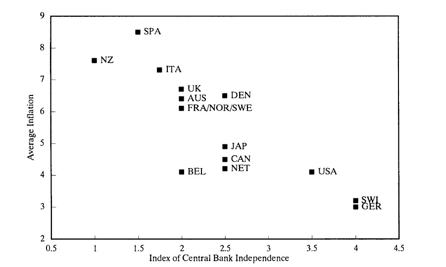
Political independence is important because a central bank that plans for the long term, rather than worrying about economic performance during election years, is more likely to maintain its commitment to low inflation. Independence from political control can therefore reassure the public about the central bank’s credibility. Influential research by Alesina and Summers (1993) showed that more independent central banks were associated with lower inflation.
Conservative central bankers may also improve outcomes. If a central banker strongly dislikes inflation, and the public believes this, the economy can move closer to the ideal low-inflation outcome without having to raise unemployment. The government may therefore appoint a central banker who is more inflation-averse than the government itself. Paul Volcker’s appointment as Fed chair in 1979 might be an example.
Consequences for bad inflation outcomes provide another way to establish credibility. Introducing laws that impose adverse consequences on central bankers when inflation is high can help convince the public that they will adhere to a low-inflation commitment.
Figure 8. Central bank independence and average inflation across countries, as reported by Alesina and Summers (1993)
16.5.5 Influence of This Research
These ideas had a considerable influence on the legal structure of central banks around the world.
Political independence has increased substantially. For example, the Bank of England was made independent in 1997; previously, the Chancellor of the Exchequer had set interest rates. The ECB/Eurosystem is also highly independent of political control.
The idea of conservative central bankers has also become influential. Central bankers around the world now speak much more about the evils of inflation and the benefits of price stability. They mainly do so because they believe these claims, but there is also a marketing element: the public’s belief in a commitment to low inflation may improve the macroeconomic tradeoff available to the central bank.
consequences for bad inflation outcomes have become more common. Many central banks have legally imposed inflation targets, with penalties or formal obligations when the target is not met. For instance, the Governor of the Bank of England must write a letter to the Chancellor explaining why the inflation target was not achieved.
16.6 Discussion of Low Inflation
16.6.1 Long-Run Benefits of Low Inflation
Because central banks now believe that they cannot reliably control unemployment or economic growth over long periods, they tend to focus on what they believe they can control: inflation. In recent years, most central banks have aimed to keep inflation low and stable as their main goal.
Former Fed chair Ben Bernanke, in his speech The Benefits of Price Stability, argued that
“the mandated goals of price stability and maximum employment are almost entirely compatible.”
Low inflation can support long-run economic growth by
- saving the time and energy associated with dealing with high inflation, such as regularly resetting prices or rewriting contracts.
- It can facilitate long-run decision-making because consumers and businesses do not need to worry as much about uncertainty concerning the future price level.
- It can also improve the price signals on which the market system relies.
However, it is difficult to argue on these grounds that there is a large welfare gain from reducing inflation from, for example, 4% to 2%.
16.6.2 Problems with a Low Inflation Target
Most central banks have adopted an inflation target of approximately 2% over the past two decades, and inflation has generally been kept in check in advanced economies since the mid-1980s.
More recently, there has been debate over whether a 2% inflation target is too low. When inflation averages 2%, relatively small shocks can bring the economy close to deflation. A higher inflation target might give central banks more room to reduce interest rates before reaching lower bounds on policy rates and having to use unconventional policies such as quantitative easing (QE).
The paper by Blanchard et al., Rethinking Macroeconomic Policy, and Ben Bernanke’s blog post The Zero Lower Bound on Interest Rates discuss the potential benefits and costs of higher inflation targets.
There have also been signs that some policy-makers are reconsidering a focus purely on inflation targeting. The Reserve Bank of New Zealand, the first pure inflation targeter in the 1990s, was given a changed mandate in March 2018 that required it also to take employment into account when making monetary policy decisions.
16.7 Inflation
16.7.1 Low Inflation Prior to 2021
Prior to 2021, inflation had been low in advanced economies for years despite many of these economies experiencing very low unemployment. Some commentators speculated that “the Phillips curve is dead,” meaning central banks no longer needed to worry about overheating economies generating higher inflation.
Several explanations were proposed.
- First, the unemployment rate may have become a poor summary measure of the balance between supply and demand in the economy.
- Second, in an increasingly globalised economy, the relevant supply capacity determining inflation may be global rather than national, with low inflation reflecting spare capacity in the world economy.
- Third, after many years of low inflation, the public’s inflation expectations may have remained anchored around 2%.
In his 2021 paper Central Banks and Inflation: Where Do We Stand and How Did We Get Here?, Karl Whelan wrote:
“the laws of supply and demand have not been repealed. There is a strong body of empirical evidence telling us that macroeconomic policy can influence aggregate demand and there is little reason to doubt that stimulating aggregate demand sufficiently can raise inflation.” Recent experience supports this view.
16.7.2 The Phillips Curve and Recent Inflation
Much of the recent surge in inflation, particularly in the euro area, was due to supply shocks, which are not part of the basic Phillips curve relationship. However, part of the increase stemmed from the effects of fiscal and monetary stimulus on aggregate demand.
The unemployment rate probably is not a very good summary measure, if it ever was, of imbalances between supply and demand. Nevertheless, central bankers have clearly continued to use the expectations-augmented Phillips curve to frame their thinking about how to reduce inflation.
Central banks such as the Fed and the ECB raised interest rates to slow economic activity and reduce inflation. They also expressed concern that high inflation could de-anchor inflation expectations, potentially leading to a return of stagflation.
However, increases in longer-term inflation expectations measured by surveys of consumers and professional economists were relatively restrained. This suggested that the public largely expected the high inflation rates to be temporary.
16.8 MMT
In the years before the pandemic, the absence of inflation and the weak relationship between money supply and prices prompted some high-profile alternative approaches to monetary policy.
The school known as Modern Monetary Theory (MMT), associated most notably with Stefanie Kelton, promotes the idea that government spending should be financed by central bank money creation rather than taxes, up to the point where such financing causes inflation.
MMT advocates are correct that this is technically a possible way to run macroeconomic policy. However, this raises important questions. Would a central bank tasked with financing government spending be sufficiently independent to restrain inflation when it rises? Would governments actually adjust spending and taxes to control inflation?
Over the long run, there is a relatively simple reason why financing government spending through central bank money creation is not a magic solution. If the government wants to increase real government spending, the required resources must come from the private sector. This transfer can happen through taxes that reduce private incomes, or through higher prices that act as an inflation tax.