14 More on Long-Term Interest Rates: Term Premia, Risk Premia and Collateral
14.1 Term Premia
Recall the expectations theory:
\[ i_{nt}=\frac{1}{n}E_t\sum_{k=0}^{n} i_{1,t+k} \]
Yield curve should only slope upwards if markets expect that short-term interest rates will be increasing. But the yield curve almost always slopes up: Markets cannot always be expecting short rates to be increasing!
Alternative: Adapt the model to allow for a positive term premium:
\[ i_{nt}=\mu_n+\frac{1}{n}E_t\sum_{k=0}^{n} i_{1,t+k} \]
where
\[ \mu_n>\mu_{n-1}. \]
Term premia may vary over time. In this case, the model is:
\[ i_{nt}=\mu_{nt}+\frac{1}{n}E_t\sum_{k=0}^{n} i_{1,t+k} \]
14.1.1 Bond Returns
For simplicity, consider a world in which the yield curve is flat, so the yield on bonds of all maturities is the same.
Consider a two-year bond issued today that pays $1,000 in two years. Its current selling price is approximately $942:
\[ P_t=\frac{\$1{,}000}{(1.03)^2}\approx\$942. \]
The yield on this bond is 3%. If yields do not change, the bond will be worth approximately $971 next year:
\[ P_{t+1}=\frac{\$1{,}000}{1.03}\approx\$971. \]
The investor will therefore earn a return of 3% over the year.
Now suppose that, at the end of the first year, yields on all newly issued bonds have jumped to 10%. The existing bond has only one year remaining until maturity. To be sold in the market, it must also offer a 10% return to the buyer, so its price must fall to approximately $909:
\[ P_{t+1}=\frac{\$1{,}000}{1.10}\approx\$909. \]
The seller has incurred a one-year return of approximately −3.4%.
The effect is far greater for a long-term bond. A ten-year bond purchased one year earlier for approximately $744 is now worth only about $424 when yields jump from 3% to 10%:
\[ P_t=\frac{\$1{,}000}{(1.03)^{10}}\approx\$744, \]
\[ P_{t+1}=\frac{\$1{,}000}{(1.10)^9}\approx\$424. \]
This represents a one-year return of approximately −43%.
14.1.2 Comparing the Riskiness of Short- and Long-Term Bonds
Now let’s compare the riskiness of long- and short-term bonds.
In favour of long-term bonds:
- Most investors have a long-term horizon and over that horizon these bonds provide a guaranteed return. Remember, in our example, the bond is guaranteed to pay $1000 at the maturity.
- They turn out to be a good investment if interest rates decline in the future.
Against long-term bonds:
- Their value is very sensitive to changes in interest rates. While risk-free if held to maturity, they are very risky investments for those with short horizons or those who may sometimes have to liquidate assets quickly.
- The guaranteed payout is usually nominal, so they will turn out to be a bad investment if inflation is higher than expected. In contrast, interest rates on short-term bonds will tend to rise with inflation, so a “rollover” strategy has less inflation risk.
On balance, these latter points appear to dominate most of the time, so the yield curve usually slopes upwards.
14.2 The Yield Curve as an Indicator of Recessions
The simple version of the expectations theory says that when the yield curve slopes up, it means that people expect interest rates to rise in the future and when it slopes down they expect interest rates to fall. Once you factor in term premia, things are not so simple. The yield curve usually slopes upwards and it rarely is flat or downward-sloping.
But if the yield curve is flat to downward-sloping that means that expectations of declining future short-term rates are strong enough to overcome the term premia factor and stop the yield curve from sloping us.
This means that a downward-sloping yield curve (sometimes called an inverted yield curve) is a strong sign that financial markets think short-term rates are going to decline. This may be because financial markets think there is going to be a recession.
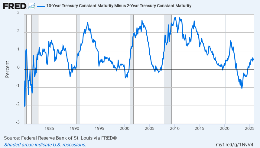
As you can see from the next graph, the ten-year Treasury yield being close to or below the two-year yield has regularly been an indicator that there will be a recession (as indicated by the shaded recession bars).
In recent years, the yield curve was inverted but a recession didn’t happen. No indicator is perfect!
Figure 1. Difference between the 10-year and 2-year US Treasury yields, with shaded US recession periods (FRED; lecture slide 8).
14.3 Risky Lending
We have discussed how monetary policy affects the benchmark interest rates on government bonds, such as US Treasury bonds. These bonds are considered essentially risk-free. These interest rates tend to influence the interest rates on all other types of lending.
If an investor can obtain an \(x\)% return on a risk-free investment over \(N\) years, then an \(N\)-year investment involving risk must offer a higher return.
We now look at risky lending: What determines the lending rates paid by corporations and households and governments?
14.3.1 Default Risk and Borrowing Rates
An alternative to investing in risk-free bonds is to lend to households and businesses (or governments) who may default on the bond, i.e. fail to pay you back as much as they should.
Suppose risk-free bonds give a return of \(S\), meaning you invest 1 and get back \(1+S\). For example, at a 2% yield, you would have \(S=0.02\).
Now consider an investment that has a return of \(R\) but a probability of complete default (no money paid back) of \(p\). This investment has:
- A probability \(1-p\) of a return of \(R\).
- A probability \(p\) of a return of \(-1\): Losing all your money.
So, the expected return is
\[ (1-p)R-p \]
To deliver the same expected return as the risk-free bond, we need
\[ (1-p)R-p=S \]
which implies
\[ R=\frac{S+p}{1-p}. \]
The formula
\[ R=\frac{S+p}{1-p} \]
implies that a higher default risk (higher \(p\)) increases the required return on the risky asset.
A higher \(p\): - Raises the numerator of the fraction, \(S+p\). - Lowers the denominator, \(1-p\).
Suppose the safe rate delivers a 2% rate of return, so \(S=0.02\). A default rate of 10% (\(p=0.1\)) requires a risky rate of return of
\[ R=\frac{0.02+0.1}{0.9} =\frac{0.12}{0.9} =0.133. \]
Even though it is 90% likely to pay out in full, the risky asset needs to have a return of 13.3% for risk-free investors to hold it, compared with 2% for the safe asset.
Default risk has a big effect on risky returns: For each percentage increase in default probability, the return rises more than one-for-one.
14.3.2 Collateral and Borrowing Rates
In some cases, the defaults associated with risky investments don’t have to mean losing all your money. For example, if a bank loans money to Janet to purchase a house, the house will usually be used as collateral to secure the loan. If Janet doesn’t pay back the loan, the bank gets the house.
Consider the case where a fraction \(c\), with
\[ 0\leq c\leq 1 \]
of the loan can be recovered from collateral.
This loan has: - A probability \(1-p\) of a return of \(R\). - A probability \(p\) of a return of \(c-1\): The collateral reduces the loss.
Re-doing the same maths, to deliver the same expected return as the risk-free bond, we need
\[ (1-p)R+p(c-1)=S \]
which implies
\[ R=\frac{S+p(1-c)}{1-p}. \]
The higher the value of the collateral, the lower the risky interest rate will be.
14.4 Risk Aversion
In the examples just discussed, investors only cared about the expected average return on their investment. In reality, people also care about risk. For investors that are risk averse, an investment that provides a guaranteed return of 5% is preferred to one that has an equal chance of returning zero or 10%.
For this reason, an investment with a default risk of \(p\) percent and no collateral will usually have to pay a risk premium of greater than \(p\).
Also, attitudes to risk from investors could change over time. During some periods, investors may be particularly averse to risk while at other times they may be willing to take more risk than usual.
For these reasons, risk premia on various types of investments can move around over time for other reasons than default risk or expected collateral values.
14.4.1 Four Types of Household Borrowing
To assess whether this framework helps to explain variations in interest rates across different categories of borrowers, consider four different types of loans to households:
- Credit Cards: No collateral. Can be used for any purpose (e.g. shopping for clothes). No set schedule for repayments apart from a small minimum monthly payment. Attractive to irresponsible borrowers who may not pay back.
- Personal Loans: No collateral. Usually screened by a bank manager as being for a particular purpose. Generally, a set schedule for repayments.
- Car Loans: The car can be used as collateral. But it’s not great collateral: Cars lose value quickly. Set schedule for repayments.
- Mortgages: The house is used as collateral and usually it’s pretty good collateral. Set schedule for repayments and people are generally very reluctant to default and lose their home.
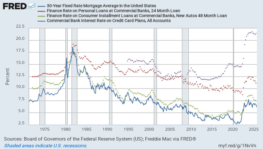
This suggests interest rates on credit cards should be the highest, then personal loans, then car loans, then mortgages. The chart below confirms that this is indeed the case.
Figure 2. US interest rates on credit cards, personal loans, car loans, and 30-year fixed-rate mortgages (FRED).
14.5 Corporate Bond Rates
Large public corporations have their credit-worthiness rated by independent ratings agencies such as Moody’s and Standard and Poor’s. Moody’s system gives the highest-rated firms get an AAA rating while firms that are an “adequate” credit risk are given a BAA rating.
Corporate bond yields tend to move in line with yields on Treasuries of similar maturities, usually around seven years. But BAA bond yields are higher than AAA rates. This reflects higher perceived default rates.
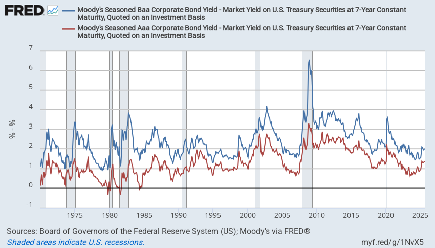
Because default risk goes up and down over the cycle, the “risk spreads(风险利差:风险资产的收益率,减去无风险资产(美国国债)收益率的差额)”associated with these bonds tend to display a cyclical pattern, rising during and after recessions, when corporate default risks are high.
These risk spreads spiked upwards to all-time highs during the period after the Lehmans bankruptcy in 2008. Spreads have actually fallen a bit over the past year despite fears of a possible upcoming recession.
Figure 3. Moody’s AAA and BAA corporate bond yields compared with the 7-year US Treasury yield (FRED).
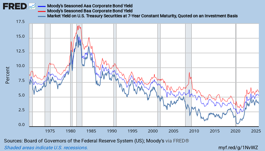
Figure 4. AAA and BAA corporate bond spreads over the 7-year US Treasury yield, with shaded US recession periods (FRED).
14.6 The Credit Channel of Monetary Policy
We have described how monetary policy affects risk-free interest rates. But to the extent that monetary policy affects household and corporate default risks, monetary policy can affect the actual borrowing rates faced by the private sector by more than the rates seen in money markets or markets for government debt.
Another issue is the effect of monetary policy on asset prices. We will not have time to discuss this issue in detail here but it is generally accepted that higher interest rates reduce the value of important assets such as house prices.
Assets like these often act as collateral in loan agreements. By influencing the value of this collateral, monetary policy can further affect risk spreads on debt.
These factors mean that central banks need to do more than just watch the money markets and the yield curve. They also need to monitor how default premia and other factors that affect borrowing rates for firms and households.
This credit channel—and the role that it played in the Great Depression—was one of Ben Bernanke’s main areas of research prior to joining the Fed.