10 Monetarism
Monetarism is a school of macroeconomic thought associated with Nobel Prize winner Milton Friedman (1912–2006). Friedman was an incredibly influential figure in academic economics and public debate on economic issues. He was both an outstanding academic and a gifted communicator of economics to popular audiences.

The essence of Friedman’s monetarist thinking was that central banks should seek to control measures of the supply of money (such as M1) so that they grow in a steady predictable manner.
Friedman’s thinking stemmed from his hugely important 1963 book, A Monetary History of the United States, co-authored with Anna J. Schwartz. The book documented that the Federal Reserve had allowed the money supply to contract significantly during the Great Depression. Friedman and Schwartz judged this to be the reason for the severity of the depression and thus wanted central banks to focus more on controlling the money supply.
Friedman’s 1970 paper “The Counter-Revolution in Monetary Theory” provides a succinct summary of his thinking about monetarism.
10.1 Monetarism in Theory
10.1.1 Quantity Theory of Money
A useful term when thinking about the role of money in the economy is velocity. The velocity of money is defined as
\[ V=\frac{PY}{M} \]
where:
- \(P\) is the GDP price index;
- \(Y\) is real GDP;
- \(M\) is the money supply.
Velocity is the amount of spending over a given period (national accounts usually measure GDP over a year) that is supported by one unit of money.
If velocity is constant, then nominal GDP is proportional to the money supply:
\[ PY=MV\quad\Longrightarrow\quad PY\propto M. \]
Most economists believe in long-run monetary neutrality, meaning that the level of real GDP is independent of the amount of money that has been supplied.
This would mean that, in the long run, the price level is proportional to the money supply:
\[ PY\propto M\quad\Longrightarrow\quad P\propto M. \]
This idea is known as the Quantity Theory of Money and was an important part of monetarist thinking.
Friedman argued that inflation is a monetary phenomenon: it can be produced by an increase in the quantity of money that is more rapid than the increase in output. He also noted that monetary growth itself can have different sources, including gold discoveries and the financing of government or private spending.
Milton Friedman (1970) on Money and Inflation:
It follows from the propositions I have so far stated that inflation is always and everywhere a monetary phenomenon in the sense that it is and can be produced only by a more rapid increase in the quantity of money than in output. However, there are many different possible reasons for monetary growth, including gold discoveries, financing of government spending, and financing of private spending
10.1.2 Some Long-Run Evidence
Many studies have examined the relationship between the money supply and inflation.
The chart on the following slide is from a speech by Isabel Schnabel, a member of the ECB Executive Board. It uses data for about 30 countries from 1951–2021, drawn from a 2023 study by BIS economists Claudio Borio, Boris Hofmann, and Egon Zakrajšek. Each dot represents the average inflation rate and excess broad money growth rate for a decade. Broad money refers to the M3 measure, and excess growth means growth above the growth rate of nominal GDP. The chart shows a strong relationship between excess money growth and inflation in the full sample.
Money Growth and Inflation: 30 Countries, 1951–2021 (Slide 9)
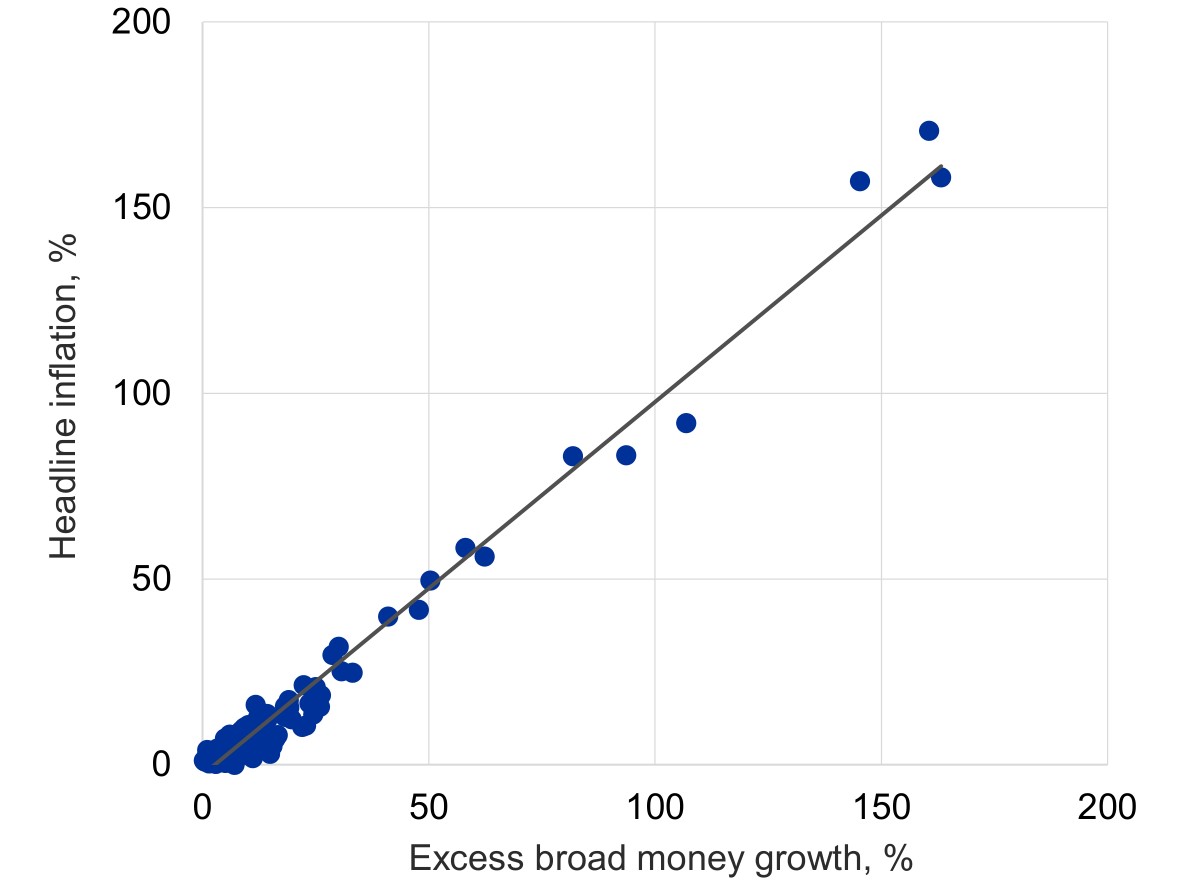
An interesting pattern often reported in studies like this is that regressions estimate the effect of money growth on inflation to be greater than predicted by the Quantity Theory: the estimated coefficient on money growth is greater than one.
10.1.3 Velocity During Periods of High Inflation
What explains why the coefficient on money growth can be greater than one? The answer is that velocity tends to increase as inflation rises. During periods of high inflation, people look to spend money as quickly as possible before it loses value.
Return to the identity:
\[ MV=PY. \]
This means that the sum of the growth rates of money and velocity equals the sum of the growth rates of prices and real GDP.
Let the growth rate of a series \(X\) be denoted by \(G_X\). Written in terms of growth rates, the quantity equation is expressed as
\[ G_M+G_V=G_P+G_Y. \]
Rearranging gives
\[ G_P=G_M+G_V-G_Y. \]
The increase in velocity during a hyperinflation explains why inflation can increase more than one-for-one with money growth: as money growth increases, velocity also increases, further raising inflation.
10.1.4 Fiscal Sources of Hyperinflations
Hyperinflation is defined as inflation above 50 percent per month. In countries with poorly developed tax systems, or in countries undergoing crises such as wars, central bank money printing often becomes the key source of government funding.
The lecture refers to a CNBC presentation, “Top 5 Hyperinflations of All Time,” and a short paper by Steve Hanke and Nicholas Krus documenting hyperinflations from world history.
Most examples of hyperinflation have stemmed from central banks providing large amounts of financing to fund government budget deficits.
10.1.5 Short-Run Implications of the Quantity Theory
Recall that if velocity is constant, nominal GDP is proportional to the money supply:
\[ PY=MV\quad\Longrightarrow\quad PY\propto M. \]
An increase in the money supply therefore raises nominal GDP. This could take the form of only the price level increasing, only real GDP increasing, or some combination of the two.
The idea of long-run monetary neutrality means that, in the end, only the price level increases following an increase in the money supply.
However, Friedman accepted that in the short run an increase in the supply of money raises real GDP, with this increase gradually reversed over time. The important point at this stage is that Friedman accepted that increasing the money supply was one way to boost the economy in the short to medium term.
Milton Friedman (1970) on Money and Output:
“One of the most difficult things to explain in simple fashion is the way in which a change in the quantity of money affects income. Generally, the initial effect is not on income at all, but on the prices of existing assets, bonds, equities, houses, and other physical capital. This effect, the liquidity effect stressed by Keynes, is an effect on the balance-sheet, not on the income account. An increased rate of monetary growth, whether produced through open-market operations or in other ways, raises the amount of cash that people and businesses have relative to other assets. The holders of the now excess cash will try to adjust their portfolios by buying other assets. But one man’s spending is another man’s receipts. All the people together cannot change the amount of cash all hold—only the monetary authorities can do that. However, as people attempt to change their cash balances, the effect spreads from one asset to another. This tends to raise the prices of assets and to reduce interest rates, which encourages spending”
The sequence described by Friedman is:
faster monetary growth → excess cash balances → portfolio adjustments toward other assets → higher asset prices and lower interest rates → increased spending.
10.1.6 Friedman’s Skepticism of Activist Policy
It might seem that Friedman’s views implied support for regularly adjusting the money supply in response to the state of the economy. However, Friedman was deeply conservative and skeptical of the role of government in the economy. He was the intellectual leader of the Chicago school, which emphasized the gains from free markets.
While he accepted that monetary policy could, in theory, be used to fine-tune the economy, he stressed the difficulties of doing so in practice. Friedman emphasized how difficult it was to diagnose, in real time, what was going on in the macroeconomy and how tricky it was to design policies to respond.
Ultimately, Friedman proposed that, except when responding to major shocks (such as wars and depressions), central banks should focus on increasing the money supply at a constant, predictable percentage rate.
The following passages from Friedman’s famous 1967 presidential address to the American Economic Association (published in 1968).
10.1.6.1 Friedman (1968) on Monetary Policy: The Limits of Fine-Tuning:
I have put this point last, and stated it in qualified terms—as referring to major disturbances—because I believe that the potentiality of monetary policy in offsetting other forces making for instability is far more limited than is commonly believed. We simply do not know enough to be able to recognize minor disturbances when they occur or to be able to predict either what their effects will be with any precision or what monetary policy is required to offset their effects. We do not know enough to be able to achieve stated objectives by delicate, or even fairly coarse, changes in the mix of monetary and fiscal policy. In this area particularly the best is likely to be the enemy of the good. Experience suggests that the path of wisdom is to use monetary policy explicitly to offset other disturbances only when they offer a “clear and present danger.”
10.1.6.2 Friedman (1968) on Monetary Policy: A Steady Money-Growth Rule
My own prescription is still that the monetary authority go all the way in avoiding such swings by adopting publicly the policy of achieving a steady rate of growth in a specified monetary total. The precise rate of growth, like the precise monetary total, is less important than the adoption of some stated and known rate. I myself have argued for a rate that would on the average achieve rough stability in the level of prices of final products, which I have estimated would call for something like a 3 to 5 per cent per year rate of growth in currency plus all commercial bank deposits or a slightly lower rate of growth in currency plus demand deposits only.⁶ But it would be better to have a fixed rate that would on the average produce moderate inflation or moderate deflation, provided it was steady, than to suffer the wide and erratic perturbations we have experienced.
10.1.6.3 Friedman (1960) From A Program for Monetary Stability, discussing constant money-growth rules:
“Like other academicians, I am accustomed to being met with the refrain, ‘It’s all right in theory but it won’t work in practice.’ Aside from the questionable logic of the remark in general, in this instance almost the reverse of what is intended is true. There is little to be said in theory for the rule that money supply should grow at a constant rate. The case for it is entirely that it would work in practice. There are persuasive theoretical grounds for desiring to vary the rate of growth to offset other factors. The difficulty is that, in practice, we do not know when to do so and by how much. In practice, therefore, deviations from the simple rule have been destabilizing rather than the reverse.”
10.2 Monetarism in Practice
Friedman’s monetarist policy called on the central bank to control the supply of money (such as M1) so it grew at a steady low rate. He believed they could do this via controlling the monetary base. This would end up leading to economic stability (nominal GDP rising at a steady rate) and low inflation.
These policy recommendations rested on three different ideas:
Predictable Money Multiplier: It would be wrong to argue that monetarists believed in the simplistic version of the money multiplier presented in the previous lecture. But they did believe that changes in the money multiplier were predictable enough that central banks could adjust the monetary base to control the broader money supply.
Predictable Velocity: Again, monetarists didn’t necessarily believe the pure quantity theory, in which velocity was constant, but they did believe velocity was predictable enough to allow central banks to link the growth rate of nominal GDP to the growth rate of the money supply.
Money and Inflation: For monetarists, inflation “was always and everywhere a monetary phenomenon” and central banks should expect a tight medium-term relationship between money growth and inflation.
Here, we will show that none of these ideas ended up working well in practice.
10.2.1 Predictable Money Multiplier
The simple money multiplier models described in the previous lecture had a strange and restrictive view of banking. For starters, the banks in the multiplier examples never have any equity capital (which would be illegal in the real world). They also treat credit creation as a mechanical process. In the model, a bank with excess reserves always wants to lend them to someone. But what if there is limited demand for credit? What if the bank decides to keep reserves at the central bank?
Many central banks now pay interest on reserves. Reserves are therefore not necessarily a worse asset than loans: they may earn a low return, but they have no credit risk and help banks manage potential liquidity problems.
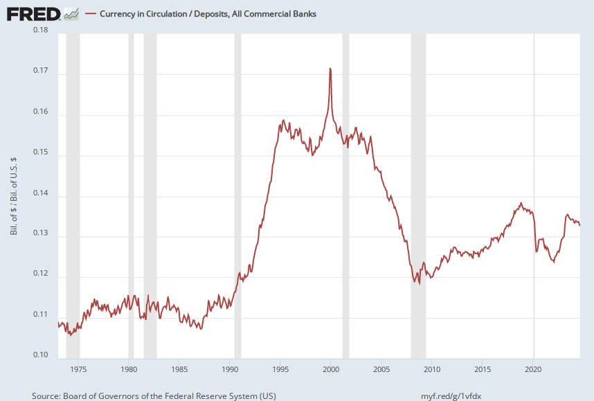
The private sector’s tendency to hold currency rather than deposits may also vary over time, affecting the multiplier.
Taken together, these complications mean that the link between the monetary base and the broader money supply is weaker than monetarists assumed.
The Ratio of Currency to Deposits in the US (Slide 22)
10.2.1.1 The Money Multiplier After QE
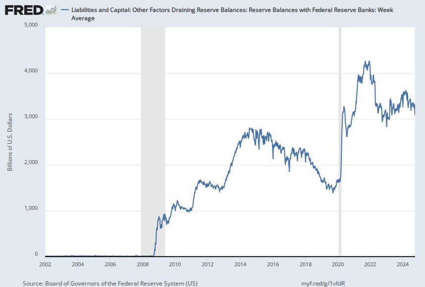
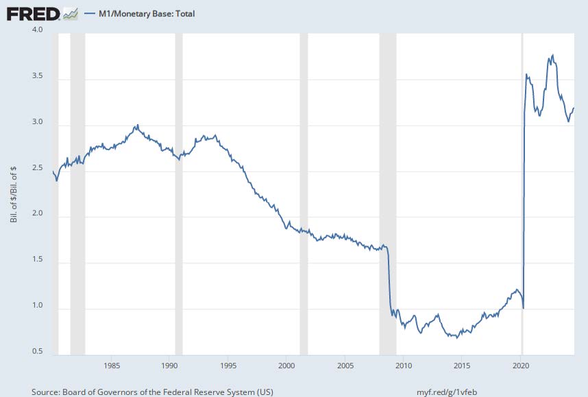
QE programs over the past decade have seen huge increases in the monetary base. During 2009 and onwards, these were not followed by proportional increases in M1 or other monetary aggregates, so money multipliers fell sharply when QE began, only partially recovering in later years: See the graph for the M1 multiplier in the US.
One explanation is there was a significant increase in the desire by banks to hold central bank reserves. During the crisis years, this may have reflected a preference for low risk investments over investments with credit risk. After the crisis, tougher liquidity regulations require banks to hold more reserves.
In 2020, the Covid pandemic saw another big increase in reserves. However, in this case, the exact opposite happened. M1 jumped up by more than M0, bringing the money multiplier back above pre-crisis levels.
The key point here: The money multiplier is not a fixed constant and how it behaves can depend on the circumstances of the economy. We cannot just assume a given increase in the monetary base will simply “multiply up” to give a broader increase in M1 or M2.
Reserve Balances of US Banks
The M1 Money Multiplier in the US
10.2.2 Predictable Velocity
The Quantity Theory was described earlier under the assumption of constant velocity. But even if velocity is not constant, monetarists argued that nominal GDP could still be controlled as long as velocity was predictable. Recall:
\[ MV=PY. \]
If the central bank knows what \(V\) will be, it can choose the appropriate \(M\) to achieve the desired level of nominal GDP.
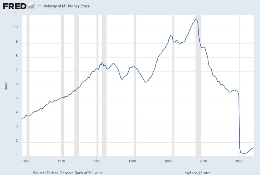
During the 1970s, M1 velocity was increasing, but in a fairly predictable fashion.
In the early 1980s, the Federal Reserve adopted the monetarist policy of targeting money-supply growth. However, the trend in M1 velocity immediately changed, and velocity has been difficult to predict since then, especially around recessions.
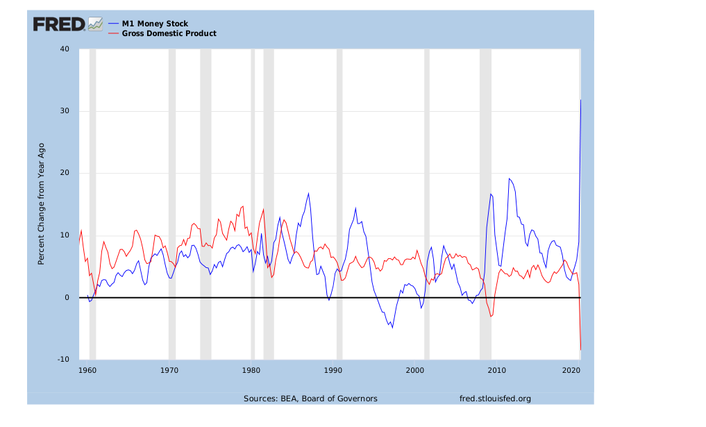
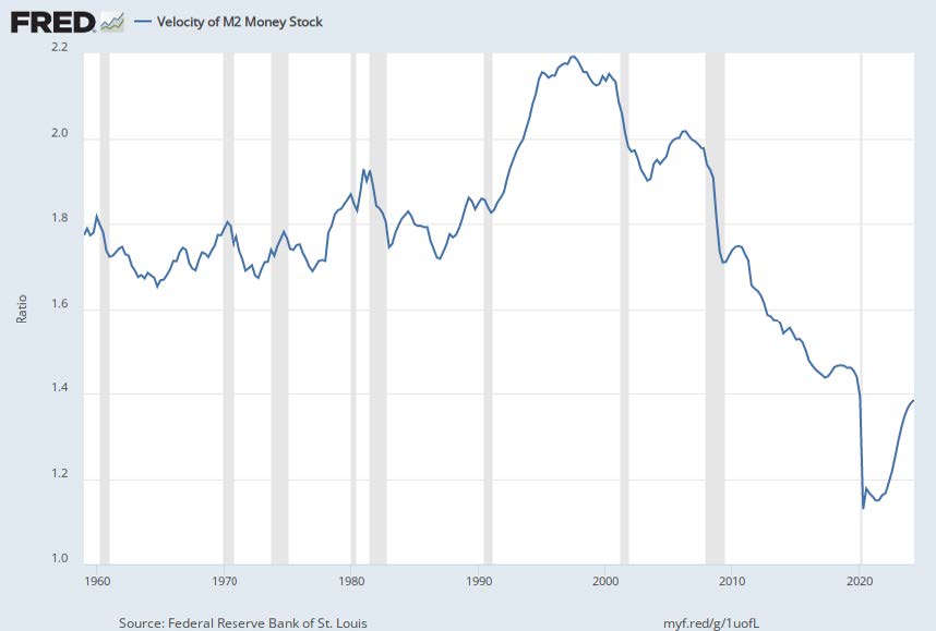
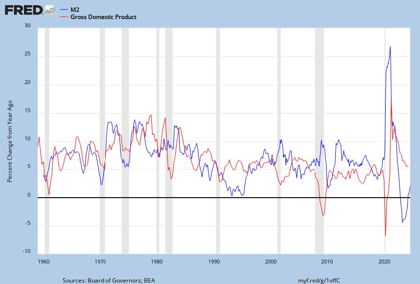
Velocity for the broader M2 measure has also been unpredictable. The relationship between money growth and nominal GDP growth, reasonably strong in the 1970s, has since been weak.
Velocity of M1 in the US
Growth Rates of M1 and Nominal GDP in the US
Velocity of M2 in the US
Growth Rates of M2 and Nominal GDP in the US
10.2.3 Money and Inflation
It isn’t too surprising that countries that turn on the printing presses to pay for government spending end up with high rates of inflation. But is money growth the key to understanding inflation in the more normal environment of countries with proper tax-raising powers and that exhibit moderate rates of inflation?
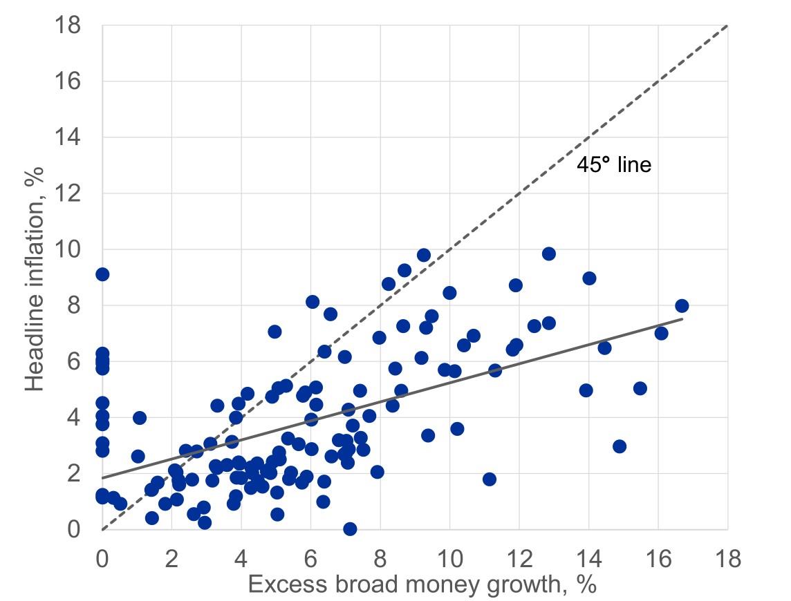
The chart (also from the Isabel Schnabel speech) shows the data from our previous chart restricted to periods with average inflation rates of below 20% per year.
The relationship is much weaker:
- The overall fit is not strong.
- There are countries with high inflation but low money growth.
- There are countries with high money growth but low inflation.
This weak relationship calls into question whether a policy based on targeting specific growth rates of the money supply is always the right way to control inflation.
Money Growth and Inflation Below 20% (Slide 32)
10.3 Example: Money and Inflation in the US
Monetarists believe that central banks can control nominal GDP via setting the correct rate of money growth.
In relation to how nominal GDP movements break down into real GDP growth and inflation, Milton Friedman was sceptical of the ability of governments to “fine-tune” the economy by controlling real GDP growth. He recommended steady growth in the money supply at a constant rate, believing that real GDP would tend to return to its natural level, so that money growth would determine the average rate of inflation.
Friedman believed that variations in the rate of money growth also tended to destabilise the real economy, so that a constant money growth rule would also deliver a more stable path for real GDP.
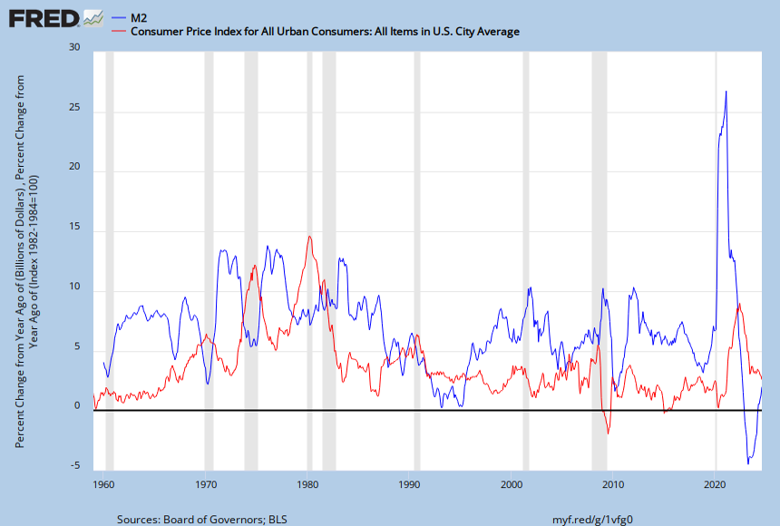
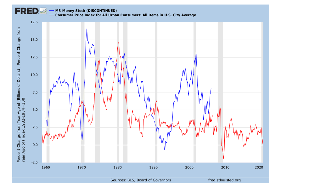
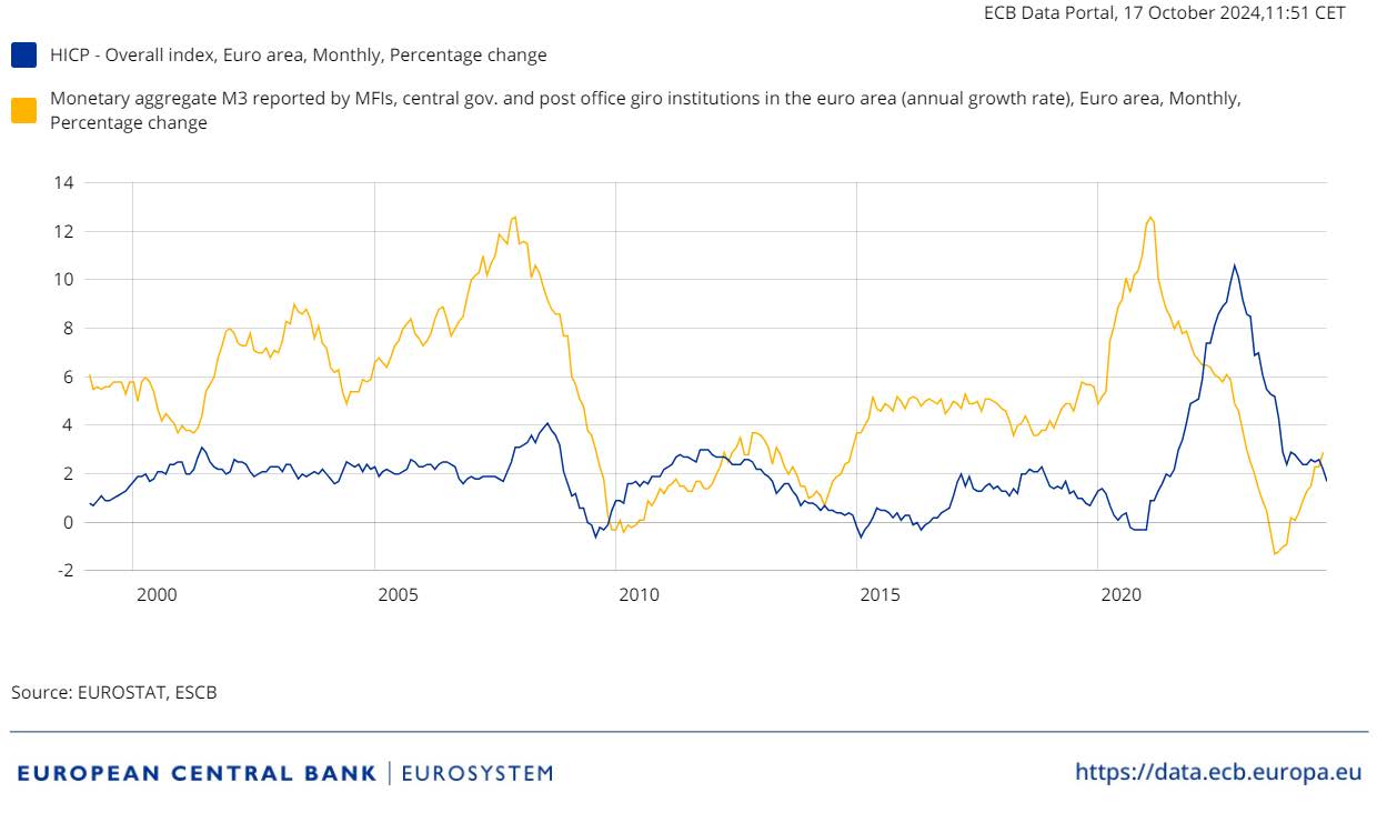
We now know that the link between money and nominal GDP growth is pretty weak these days. As for the relationship between money growth and inflation, the charts on the next show that it is hard to find a good relationship between inflation and any US measure of money growth.
US Inflation and M2 Growth
US Inflation and M3 Growth
Euro Area Inflation (Blue Line) and M3 Growth (Yellow Line)
10.4 Conclusion
To summarise, a policy of manipulating the monetary base with the aim of targeting the growth rate of the money supply is now generally considered a poor strategy for central banks for a number of reasons:
Uncertain Money Multiplier: While central banks can control the monetary base, the relationship between this base and the money supply is uncertain and depends upon unpredictable behavioural elements in the banking system.
Uncertain Monetary Velocity: Even if the central bank could control the money supply, the link between this and nominal GDP posited in the Quantity Theory requires that velocity be predictable. In reality, velocity has often been unpredictable.
Weak Link Between Money and Inflation: Stable velocity and long-run monetary neutrality are supposed to lead to a tight relationship over time between inflation and the growth rate of money. In most modern economies, this relationship just isn’t there.
In addition, as we will discuss soon, evidence from the early 1980s showed that a policy of monetary targeting leads to sharp and volatile movements in short-term interest rates.